How NTDBs Make Decisions Without a Transformer

Part II of our series on building Patronus Ark for CPU-based AI security inference.

In Part I, we gave a simplified description of Layer 2: NTDBs make the cheap decision, and Lion Warden only runs when more depth is needed.

The interesting part is how that cheap decision is built. Layer 2 cannot just be a smaller copy of Layer 3. Loading another transformer would bring back the memory and latency problems we were trying to remove. But reducing Layer 2 to a confidence score from one small classifier would not give us enough information to decide whether Layer 3 is actually needed.

NTDBs are our answer to that problem.

The name stands for Non-Transformer Decision Block. The classifiers inside an NTDB do not use transformer layers. The block can still use attention across chunks; attention alone does not make an architecture a transformer.

In the current Ark pipeline, the input is tokenized and embedded through the shared mmBERT stack. Layer 2 mean-pools the static token embeddings into one 384-dimensional vector per chunk. The token-level representation remains available for chunks that later continue through Lion Warden's contextual layers. From the pooled vector, an NTDB combines small neural components with classifiers such as LightGBM and logistic regression. It produces an L2 result and a much larger feature representation for the Promote Gate without executing Lion Warden's 22 contextual layers.

Why the decision starts with chunks

Ark processes inputs in windows of up to 256 tokens because security signals are often local. A file with 30,000 tokens can contain one short injected instruction. The surrounding benign content must not average that signal away.

The second reason is execution.

Once a chunk has been embedded, it is a vector. A document with N chunks is therefore no longer a sequence of N separate text-classification requests. It is a matrix of chunk vectors that can be passed through Layer 2 together.

This matters on a CPU. We pay much of the execution overhead once and use optimized matrix operations instead of invoking every classifier separately for every chunk. In our measurements, the resulting wall-clock time scales considerably better than serial chunk-by-chunk execution. We do not claim a different asymptotic complexity; the gain comes from processing the chunk matrix efficiently.

Chunking therefore gives us both properties we need: local security evidence stays visible, while long inputs remain efficient enough to process on a CPU.

Why Layer 2 uses the mmBERT representation

LightGBM and logistic regression do not require embeddings. A LightGBM classifier could also be trained on a sparse N-gram or TF-IDF matrix. That would still be a valid Layer-2 classifier.

It would not give us the architecture we need for Ark.

Our NTDBs use the same tokenizer, embedding layer, dimensions and latent space as Lion Warden. We tokenize and embed once. Layer 2 consumes a mean-pooled 384-dimensional view of each chunk, while promoted chunks retain the token-level embeddings required by the deeper mmBERT layers. No second tokenizer, vocabulary or embedding model has to be loaded.

The memory and latency savings are substantial, but the shared latent space is not only an optimization. It is part of the promotion problem itself.

The Promote Gate is supposed to learn whether additional depth will change a decision, not whether two unrelated feature systems happen to disagree. Layer 2, Layer 3 and the gate therefore need to operate on compatible representations of the same input. Otherwise, representation shift becomes mixed into the routing decision.

This is also where the architecture connects to statistical learning theory. We restrict the hypothesis and decision space instead of asking the promoter to compare arbitrary models with arbitrary representations. The underlying coordinates remain shared; what changes is the amount of contextual computation applied to them. This makes the learned boundary between "L2 is sufficient" and "L3 adds useful information" substantially better defined.

What an NTDB head actually computes

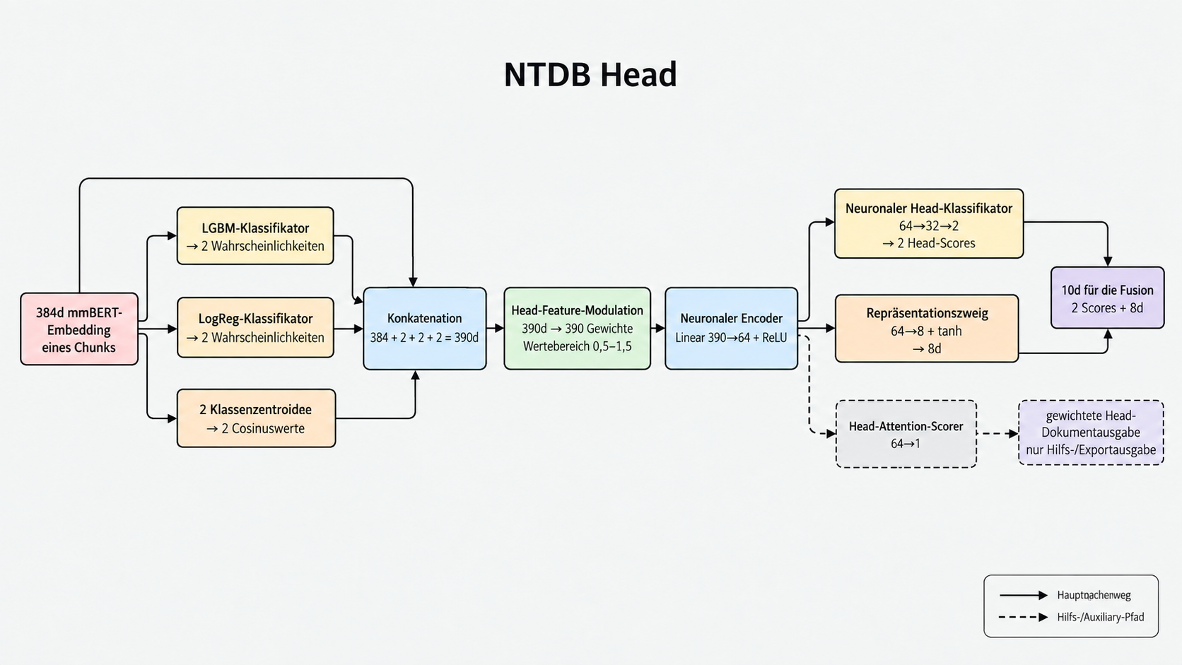
The 384-dimensional static mmBERT embedding is only the starting point. In the current Injection architecture, one NTDB head evaluates it through a LightGBM classifier, logistic regression and two class centroids. The two classifiers contribute two probabilities each; the centroids contribute two cosine similarities. Together with the original embedding, this produces a 390-dimensional input for the neural part of the head.

The next step is feature modulation. Instead of treating all 390 dimensions as equally useful for every chunk, the head learns a context-dependent weight for each feature. The modulated vector is projected to 64 dimensions. From there, the head produces two class scores and a compact eight-dimensional representation. The output of one head is therefore ten dimensions, not merely a final confidence score.

One NTDB head. The solid line is the per-chunk runtime path. The dashed attention branch produces a weighted head-level document output for auxiliary or export use; it is not the final Ark document aggregation.

Ark currently runs three such heads per Injection chunk: the Patronus head, the Jayavibhav head and an L3-surrogate head. Their three ten-dimensional outputs are concatenated into 30 dimensions, modulated again and passed through a small fusion encoder. This produces the fused L2 representation and the final L2 probability for that chunk.

For multiclass pipelines, additional NTDB heads can implement one-vs-rest decisions. That is a decomposition choice for the classification task. More heads are not an automatic mechanism for reducing false positives, and different pipelines can use different head layouts while retaining the same basic block contract.

There is attention in the exported architecture, but its role needs to be kept separate from the main runtime path. A head can score and weight representations across chunks to form a global auxiliary output. When the runtime evaluates a single chunk, there is nothing meaningful to attend over: the 64-dimensional representation is passed through unchanged and a softmax over one element is trivially one. The selective L2/L3 decision remains per chunk, and the final document decision is still a simple aggregation after promotion.

The NTDB output is not a document verdict

Layer 2 does not first decide whether the complete document is safe and then route the document to Layer 3. It produces a decision state for each chunk. In the current Injection pipeline, the separate LightGBM promoter receives 1,886 features per chunk.

The Promote Gate works on that representation and decides which chunks need Lion Warden. A chunk that is not promoted keeps its L2 result. A promoted chunk continues through Layer 3 and receives the Lion Warden result.

Only after this routing step are the chunk results combined:

shared chunk matrix
  → three NTDB heads per chunk
  → 30d head fusion → 64d fused representation
  → L2 result and 1,886 promoter features per chunk
  → Promote Gate
      ├─ keep L2 result
      └─ execute L3 and use Lion Warden result
  → aggregate selected chunk results

For evaluation, we distinguish between L2-only, L3-only and Union. Union is the actual selective path: L2 results remain for non-promoted chunks, while promoted chunks contribute their L3 results.

The final document aggregation is intentionally simple. Depending on the pipeline and operating point, Ark uses functions such as max, mean or smoothmax, followed by a learned threshold. There is no second attention mechanism hiding at the end of the pipeline.

What Layer 2 changes

NTDBs do not replace Lion Warden. They stop Ark from treating every chunk as if it required the full model.

Their useful output is not just a cheap prediction. For every chunk, Layer 2 exposes enough of its decision state for a separate model to estimate whether additional contextual computation is worth running. A confidence threshold cannot answer that reliably. L3 may correct L2, confirm it or replace a correct result with a worse one.

Part III examines this overlapping decision space and the Promote Gate trained on it. That is also where the current latency, promotion-rate and quality results belong.